Tutorial: solving and visualizing a complex ODE
This tutorial walks through solving a single complex-valued ODE with
solve_complex_ivp() and visualizing the result, reproducing an
example from the Wolfram Language documentation.
Attribution
The example problem and the idea of visualizing its solution come from
Solutions of Complex ODEs
in the Wolfram Language 12 documentation, where it is solved with
NDSolveValue.
The problem
We want to integrate the scalar, time-dependent complex ODE
The right-hand side is a (time-dependent) complex coefficient multiplying
y, so it is holomorphic in y. That is exactly the setting ZVODE is
built for: it advances the complex state directly, with no need to split the
problem into real and imaginary parts.
A reference solution
This problem is separable and has a closed-form solution, which is handy for
checking accuracy. From y'/y = 10\, e^{2\pi i t} we integrate to obtain
Since \(e^{2\pi i t} = 1\) whenever t is an integer, the exponent
vanishes there and the solution returns to y = 1 at every integer time; in
particular y(5) = 1.
Step 1 — define the right-hand side
The right-hand side takes the time t and the state vector y (here of
length 1) and returns y'. We write it to return a one-element list:
import numpy as np

def rhs(t, y):
    # y'(t) = 10 e^{2πi t} y(t)
    return [10.0 * np.exp(2j * np.pi * t) * y[0]]
Because the coefficient does not depend on y, the Jacobian
\(\partial f/\partial y = 10\, e^{2\pi i t}\) is trivial, and for this
non-stiff problem we do not need to supply it.
Step 2 — integrate
solve_complex_ivp() is the recommended entry point. The problem
is non-stiff (a smooth, oscillatory coefficient), so we select the Adams
method. Passing tspan as a full array of times requests the solution on
that grid, which makes the parametric plot below smooth:
from zvode import solve_complex_ivp

t_eval = np.linspace(0.0, 5.0, 501)

sol = solve_complex_ivp(
    fun=rhs,
    tspan=t_eval,
    y0=[1.0 + 0.0j],
    method="Adams",
    rtol=1e-10,
    atol=1e-12,
)

y = sol.y[0]   # complex array, shape (501,)
We can confirm the result against the closed form:
def exact(t):
    t = np.asarray(t, dtype=float)
    return np.exp((10.0 / (2j * np.pi)) * (np.exp(2j * np.pi * t) - 1.0))

err = np.max(np.abs(y - exact(t_eval)))
print(f"Max absolute error: {err:.2e}")   # ~9e-09
Step 3 — visualize
The Wolfram example draws the solution two ways. Each is a few lines of Matplotlib.
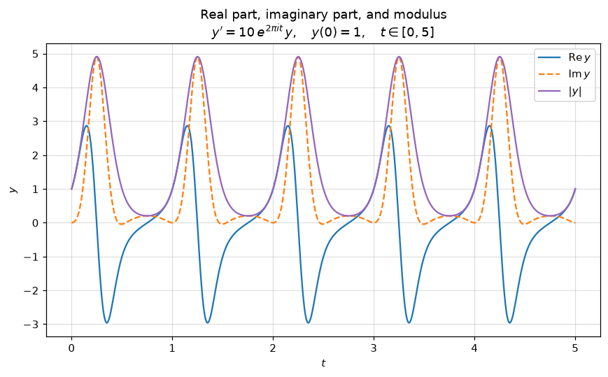
The real part, imaginary part, and modulus versus the real variable t.
Plotting all three together shows the oscillation and its envelope at a glance;
the modulus peaks near |y| ≈ 5 once per period and returns to 1 at every
integer t:
import matplotlib.pyplot as plt

plt.plot(t_eval, y.real, label=r"$\mathrm{Re}\,y$")
plt.plot(t_eval, y.imag, "--", label=r"$\mathrm{Im}\,y$")
plt.plot(t_eval, np.abs(y), label=r"$|y|$")
plt.xlabel("$t$")
plt.legend()
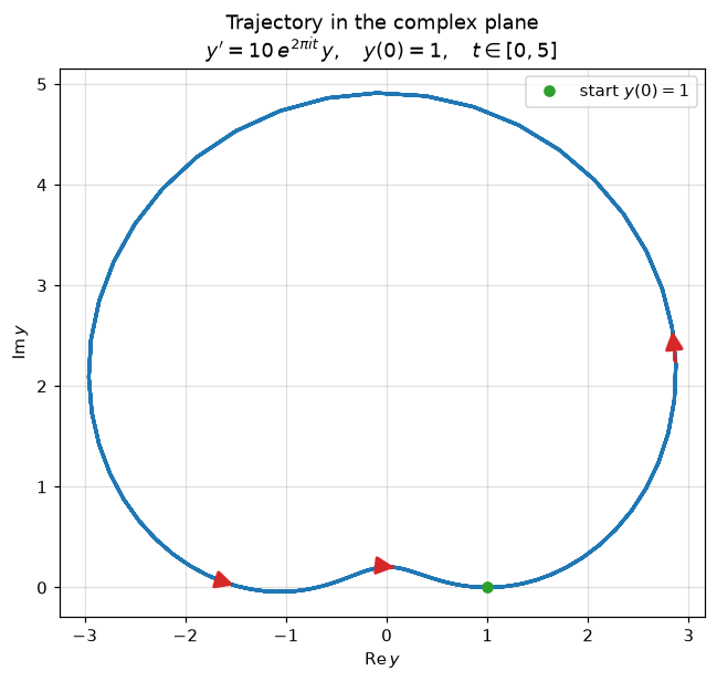
The trajectory drawn parametrically in the complex plane. Plotting
y.imag against y.real traces the path the solution follows. Because the
solution is periodic with period 1, the curve is retraced five times over
t ∈ [0, 5], so a single loop is all that is visible. A couple of arrows
(drawn with annotate() between successive sample
points) mark the direction of travel:
ax = plt.gca()
ax.plot(y.real, y.imag, linewidth=2)
ax.set_aspect("equal")

# Arrows indicating the direction of travel along the curve.
period = len(t_eval) // 5  # samples per unit-time period
for frac in (0.15, 0.45, 0.78):
    i = int(frac * period)
    ax.annotate(
        "",
        xy=(y.real[i + 1], y.imag[i + 1]),
        xytext=(y.real[i], y.imag[i]),
        arrowprops=dict(arrowstyle="-|>", color="tab:red",
                        lw=2, mutation_scale=22),
    )

ax.set_xlabel(r"$\mathrm{Re}\,y$")
ax.set_ylabel(r"$\mathrm{Im}\,y$")
The complete, runnable script is demo_complex_ode.py.
Next steps
Output modes, method selection, and supplying a Jacobian are covered in Procedural API — solve_complex_ivp.
For larger or stiff systems, see Banded Jacobians and Compiled callbacks.